Cost Functions

What is a Cost Function?

A cost function (also called a loss function or objective function) is a mathematical measure that quantifies how wrong a model’s predictions are compared to the actual values. It essentially tells us “how much our model costs us” in terms of prediction errors. The goal in machine learning is to minimise this cost by finding the optimal model parameters.

The Squared Error Cost Function

Looking at the following formula:

$$J(w,b) = \frac{1}{2m} \sum_{i=1}^{m} (\hat{y}^{(i)} - y^{(i)})^2$$

Let me break down each component:

• $J(w,b)$: The cost function value, dependent on parameters $w$ (weight) and $b$ (bias)
• $m$: The number of training examples
• $\hat{y}^{(i)}$: The predicted value for the i-th example ($\hat{y}^{(i)} = f_{w,b}(x^{(i)}) = wx^{(i)} + b$)
• $y^{(i)}$: The actual/true value for the i-th example
• $(\hat{y}^{(i)} - y^{(i)})$: The error for a single prediction
• $\sum$: Sum over all $m$ training examples
• $\frac{1}{2m}$: A normalization factor (the $\frac{1}{2}$ is often included to simplify derivatives during optimization)

Visual Interpretation

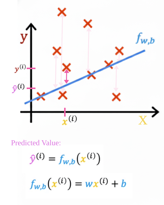This image illustrates the squared error cost function, one of the most fundamental concepts in machine learning, particularly for regression problems.

The graph shows:

• Red X’s: Actual data points $(x^{(i)}, y^{(i)})$
• Blue line: The linear model $f_{w,b} = wx + b$
• Pink arrows: The errors between predictions and actual values

The cost function calculates the average of the squared lengths of these pink arrows. Squaring serves two purposes:

1. Makes all errors positive (so they don’t cancel out)
2. Penalizes larger errors more heavily than smaller ones

The Optimization Goal

Find $w,b$ so that $\hat{y}^{(i)}$ is close to $y^{(i)}$ for all $(x^{(i)}, y^{(i)})$.

The objective is to find the optimal values of $w$ and $b$ that minimize $J(w,b)$, which means finding the line that best fits the data points with the smallest overall squared error. This is typically done using optimization algorithms like Gradient Descent.

This particular cost function leads to what’s known as ordinary least squares regression when used with linear models, forming the foundation for many more complex machine learning algorithms.

Source: Machine Learning Specialization on Coursera