Examples of Logistic Regression
 This image provides an excellent visual explanation of logistic regression and how it transforms linear outputs into probabilities.
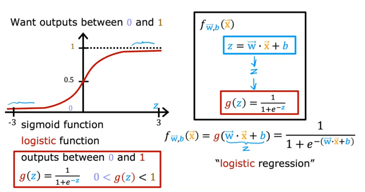
Key components illustrated:
-
The Sigmoid/Logistic Function (left graph):
- Shows the characteristic S-shaped curve that maps any real number to a value between 0 and 1
- The x-axis represents the linear combination z (ranging from -3 to 3 in this example)
- The y-axis shows the output probability (0 to 1)
- At z=0, the output is exactly 0.5 (the midpoint)
- As z approaches negative infinity, the output approaches 0
- As z approaches positive infinity, the output approaches 1
-
The Mathematical Flow (right side):
- First, a linear combination is computed: z = w·x + b
- w represents the weights (parameters)
- x represents the input features
- b represents the bias term
- Then, this linear value z is passed through the sigmoid function: g(z) = 1/(1+e^(-z))
- This transformation ensures the final output is always between 0 and 1
- First, a linear combination is computed: z = w·x + b
-
The Complete Model:
- The bottom equation shows the full logistic regression model: f(x) = 1/(1+e^(-(w·x+b)))
- This combines both steps into a single function
Why this transformation matters:
- Linear regression could produce any value (negative, greater than 1, etc.)
- For classification, we need probabilities bounded between 0 and 1
- The sigmoid function provides this smooth, differentiable transformation
- The resulting probabilities can be interpreted as the likelihood of belonging to the positive class
This visualization effectively demonstrates why logistic regression is called “logistic” - it uses the logistic (sigmoid) function to convert unbounded linear predictions into valid probability values.
Related
- Gradient Descent - The optimisation algorithm used to train logistic regression models
- Supervised Learning - Logistic regression is a supervised classification algorithm